Goals

The examples below are meant to show you how to implement the three options for regression when you are violating the normality and/or equal variance assumptions:

Remove outliers
Transform the data
Use a non-parametric model (Theil-Sen regression)

Example 1: Removing outliers

This dataset was generated by recording the miles traveled and kwh consumed each day, and recording the average temperature for the day from a local weather service. The question guiding our example is: How does ambient temperature affect an electric car’s efficiency + range?

library(tidyverse)
library(MASS)
library(mblm)

ecar <- read.csv("./data/ecar-and-temp-clean.csv") 
str(ecar)

'data.frame':   54 obs. of  3 variables:
 $ date  : chr  "11/1/21" "11/3/21" "11/4/21" "11/6/21" ...
 $ mi_kwh: num  3.42 3.52 3.28 2.91 2.87 ...
 $ temp_F: num  58.4 55 51.4 48 47.2 48.2 54.4 51.2 57.6 55.8 ...

Examine scatterplot

# Use ggplot to create a scatterplot to visualize the relationship between the two variables, putting the independent variable on the x axis and the dependent on the y axis

ggplot(data = ecar, aes(x = temp_F, y = mi_kwh)) +
  geom_point() +
  theme_bw() +
  labs(x = "Temperature (deg F)", y = "Miles per kwh charge")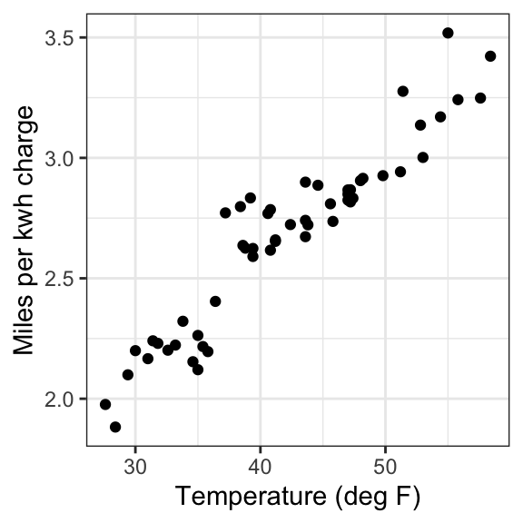

Fit a linear regression model + assess assumptions

Use the function lm() to fit a linear regression model of mi/kwh as a function of temperature. The function requires the following arguments:

formula: a description of the model to be fitted (form: y ~ x)
data: the name of the data frame containing the variables in the formula

mod <- lm(mi_kwh ~ temp_F, data = ecar)

# Let's check the fit using diagnostic plots...
par(mfrow=c(2,2))
plot(mod)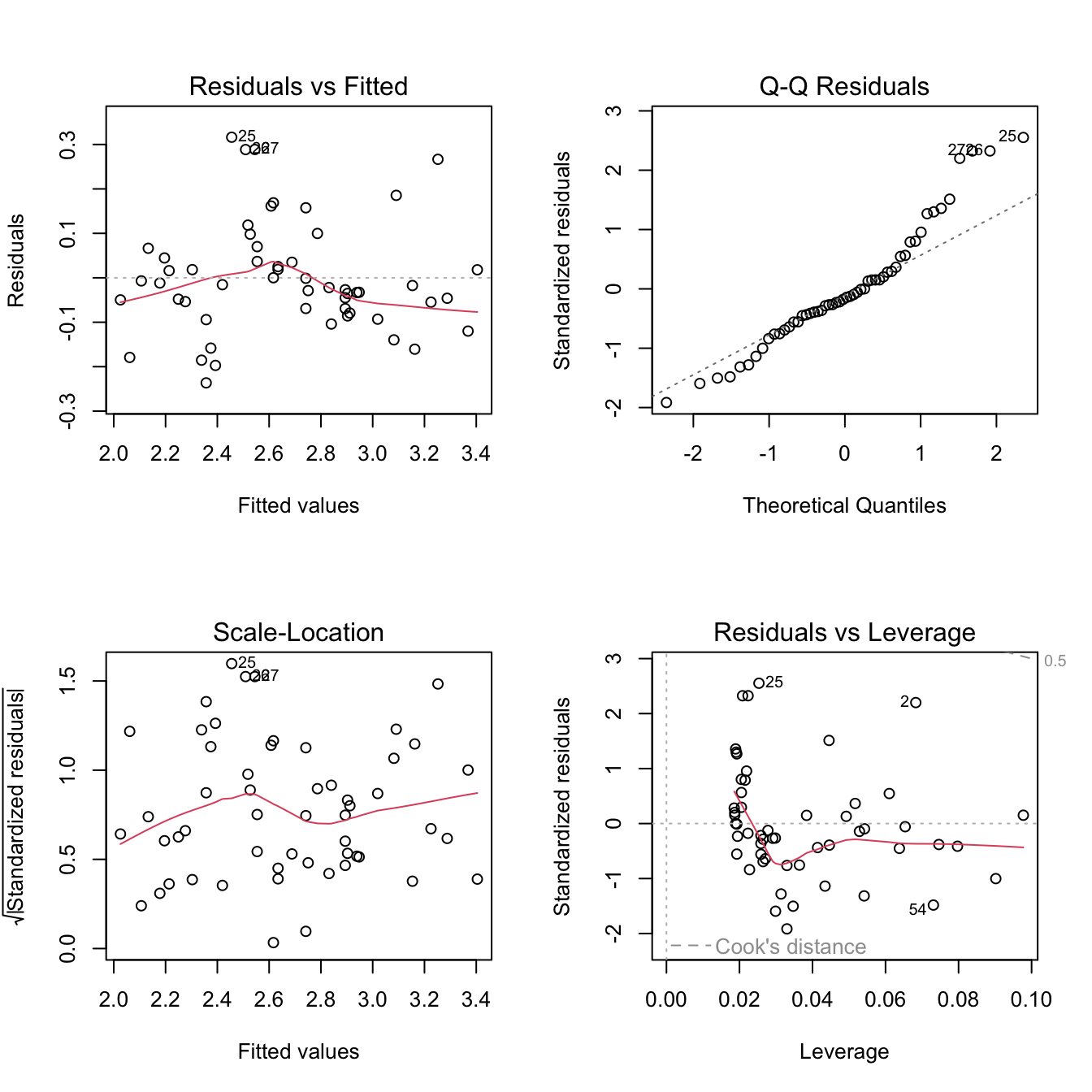

# And a histogram of the residuals...
hist(mod$residuals)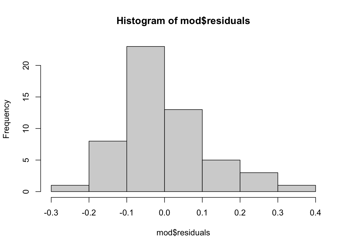

# Check mean and median of residuals
# Mean will always be zero, median may not be if not normal...
# We can see that the median is slightly below zero...
round(mean(mod$residuals), digits = 2)

[1] 0

round(median(mod$residuals), digits = 2)

[1] -0.02

# Create a new dataframe with the outliers marked
# First create a variable to store the row numbers
# Then use mutate + ifelse to mark the outliers
ecar_mark <- ecar %>%
  mutate(rownum = seq(from = 1, to = 54, by = 1),
         col = ifelse(rownum %in% c(25, 26, 27), "outlier", "not outlier"))

# Plot again with outliers marked
ggplot(data = ecar_mark, aes(x = temp_F, y = mi_kwh, colour = col)) +
  geom_point() +
  theme_bw() +
  labs(x = "Temperature (deg F)", y = "Miles per kwh charge") +
  theme(legend.title=element_blank(), legend.position = "top") +
  scale_colour_manual(values = c("black","blue"))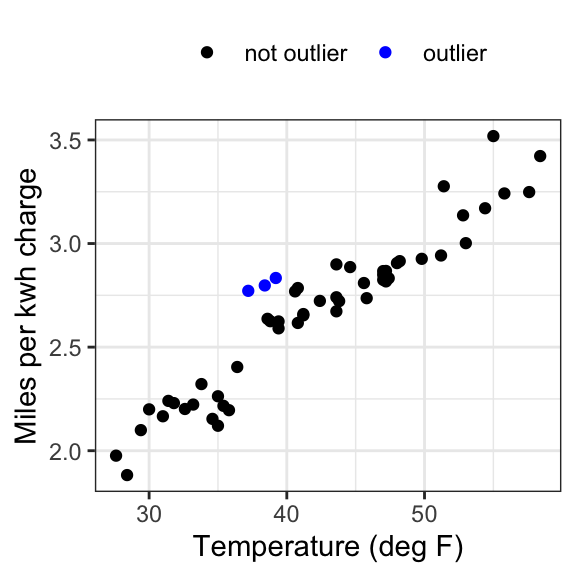

Exclude outliers + re-fit the model

We can see that there are a few potential outliers in our dataset (rows 25, 26, 27 - frequently marked as such on the diagnostic plots). These do not look too extreme, but if we are worried about them, we can refit the model without those points to see if it changes the outcome.

# To remove those rows from the data we will use a skill called 'indexing'
# The negative sign indicates we want to remove rows 25, 26, 27
# The comma after the parenthesis is important - 
# leaving the second part blank selects all columns
ecar_no_outliers <- ecar[-c(25,26,27), ]

# Now let's refit the model...
mod_no_outliers <- lm(mi_kwh ~ temp_F, data = ecar_no_outliers)

# Since we created a column, we can easily filter
ecar_no_outliers <- ecar_mark %>%
  filter(col != "outlier") # notice the exclamation point! (means 'not')

# Now let's refit the model...
mod_no_outliers <- lm(mi_kwh ~ temp_F, data = ecar_no_outliers)

# And check the fit...
par(mfrow=c(2,2))
plot(mod_no_outliers)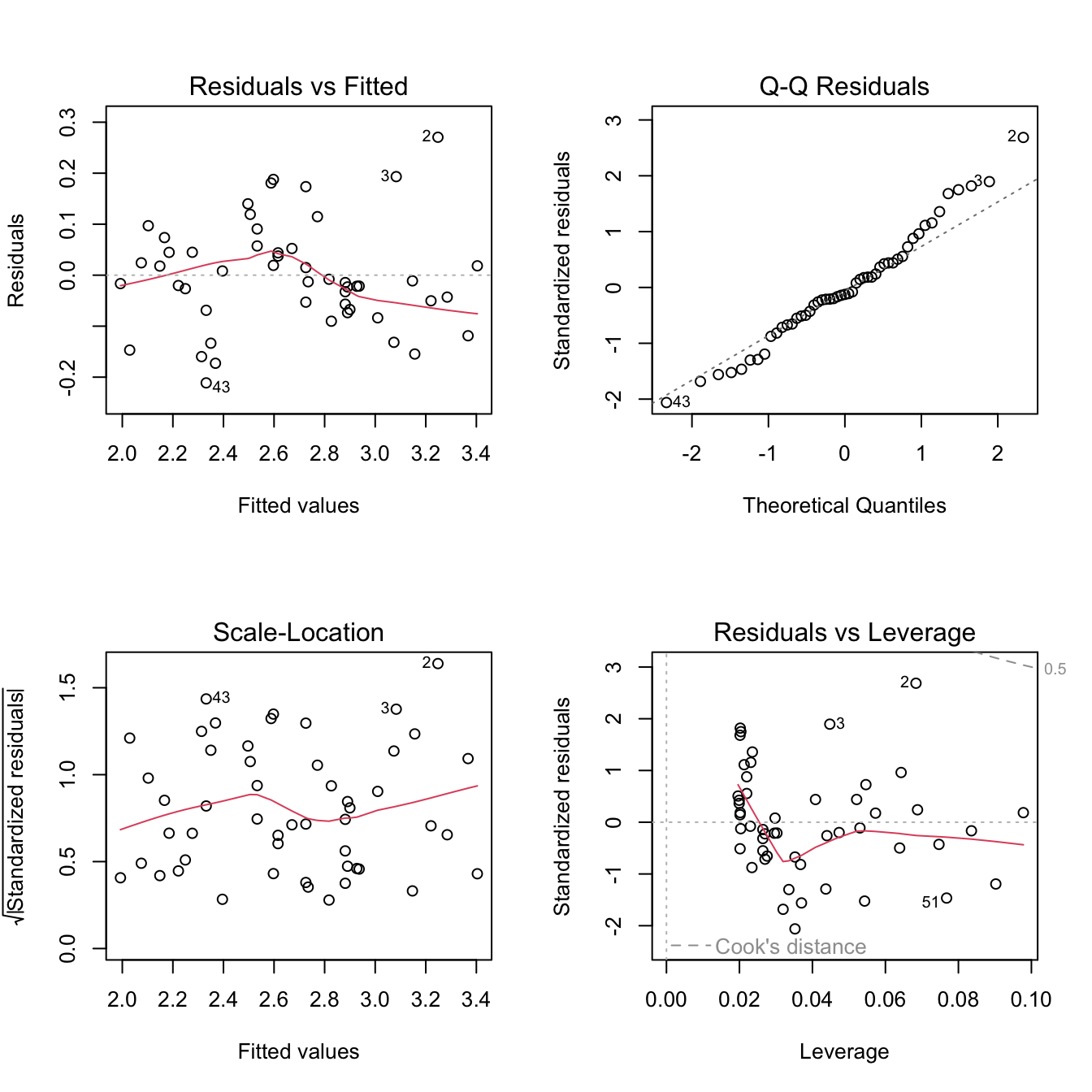

hist(mod_no_outliers$resid)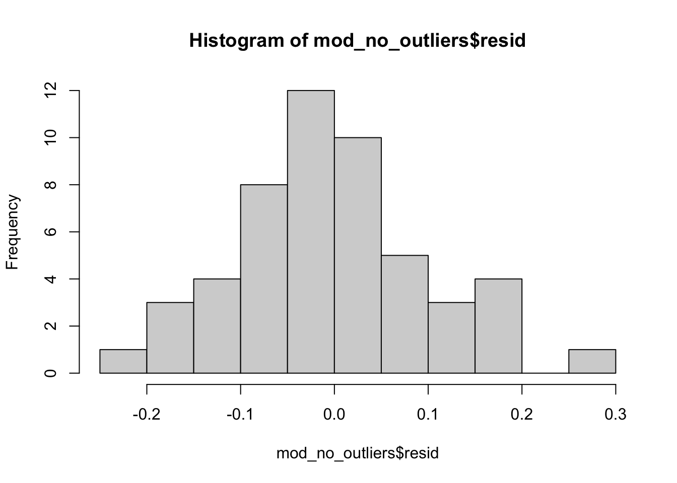

Compare models

Do your conclusions change?

summary(mod)


Call:
lm(formula = mi_kwh ~ temp_F, data = ecar)

Residuals:
     Min       1Q   Median       3Q      Max 
-0.23648 -0.06920 -0.01967  0.04267  0.31633 

Coefficients:
            Estimate Std. Error t value Pr(>|t|)    
(Intercept) 0.790601   0.092151   8.579 1.56e-11 ***
temp_F      0.044753   0.002156  20.761  < 2e-16 ***
---
Signif. codes:  0 '***' 0.001 '**' 0.01 '*' 0.05 '.' 0.1 ' ' 1

Residual standard error: 0.1255 on 52 degrees of freedom
Multiple R-squared:  0.8923,    Adjusted R-squared:  0.8903 
F-statistic:   431 on 1 and 52 DF,  p-value: < 2.2e-16

summary(mod_no_outliers)


Call:
lm(formula = mi_kwh ~ temp_F, data = ecar_no_outliers)

Residuals:
     Min       1Q   Median       3Q      Max 
-0.21124 -0.06210 -0.01290  0.04861  0.27054 

Coefficients:
            Estimate Std. Error t value Pr(>|t|)    
(Intercept) 0.728025   0.077560   9.387 1.58e-12 ***
temp_F      0.045820   0.001804  25.401  < 2e-16 ***
---
Signif. codes:  0 '***' 0.001 '**' 0.01 '*' 0.05 '.' 0.1 ' ' 1

Residual standard error: 0.1043 on 49 degrees of freedom
Multiple R-squared:  0.9294,    Adjusted R-squared:  0.928 
F-statistic: 645.2 on 1 and 49 DF,  p-value: < 2.2e-16

Example 2: Transformation

In the previous example, our data reasonably fit the assumptions. Now let’s look at an example where that is not the case and see how we might adjust the data to meet assumptions.

We will use a dataset called mammals that contains average brain weights (in g) and body weights (in kg) for 62 species of land mammals. We want to know if mammals with heavier bodies also have heavier brains.

Preliminary plots

# Use ggplot to examine the relationship between body weight and brain weight
ggplot(data = mammals, aes(x = body, y = brain)) +
  geom_point(alpha = .5) +
  theme_bw() +
  labs(x = "Body weight (kg)", y = "Brain weight (g)")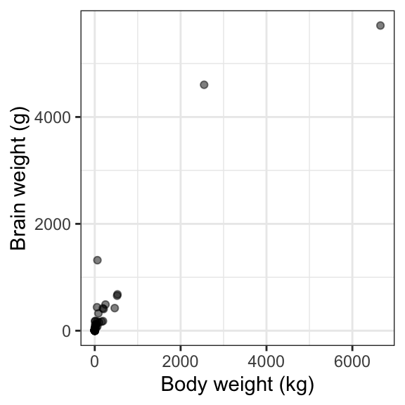

# Use ggplot to examine the histograms for each variable
ggplot(data = mammals, aes(x = body)) +
  geom_density() +
  theme_bw()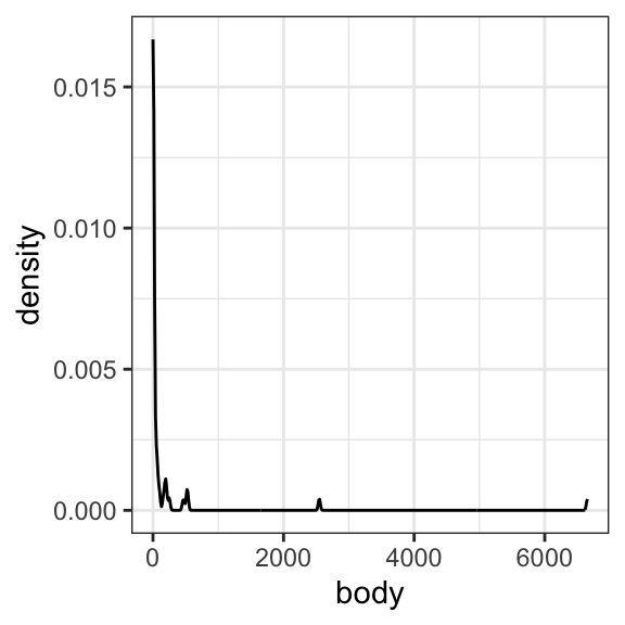

ggplot(data = mammals, aes(x = brain)) +
  geom_density() +
  theme_bw()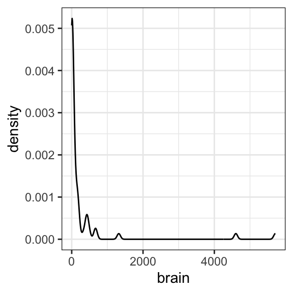

Fit a linear regression model + assess assumptions

Now let’s see what happens when we fit a linear model to these data.

mod_raw <- lm(brain ~ body, data = mammals)

par(mfrow=c(2,2))
plot(mod_raw)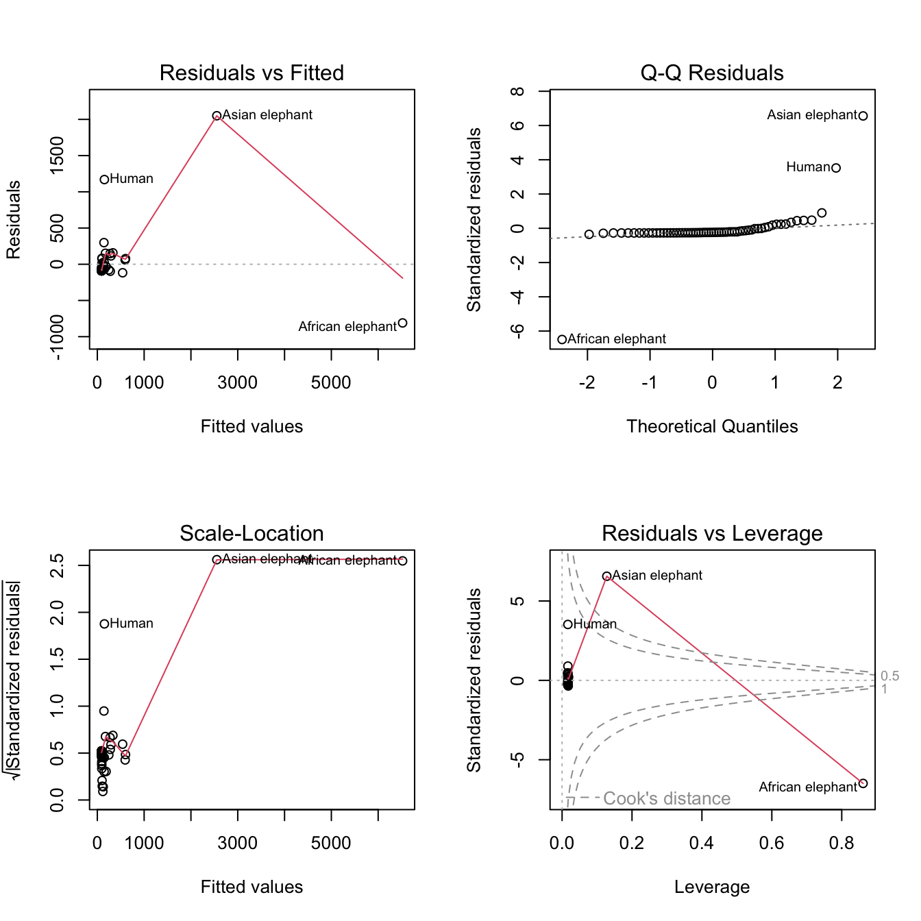

hist(mod_raw$residuals)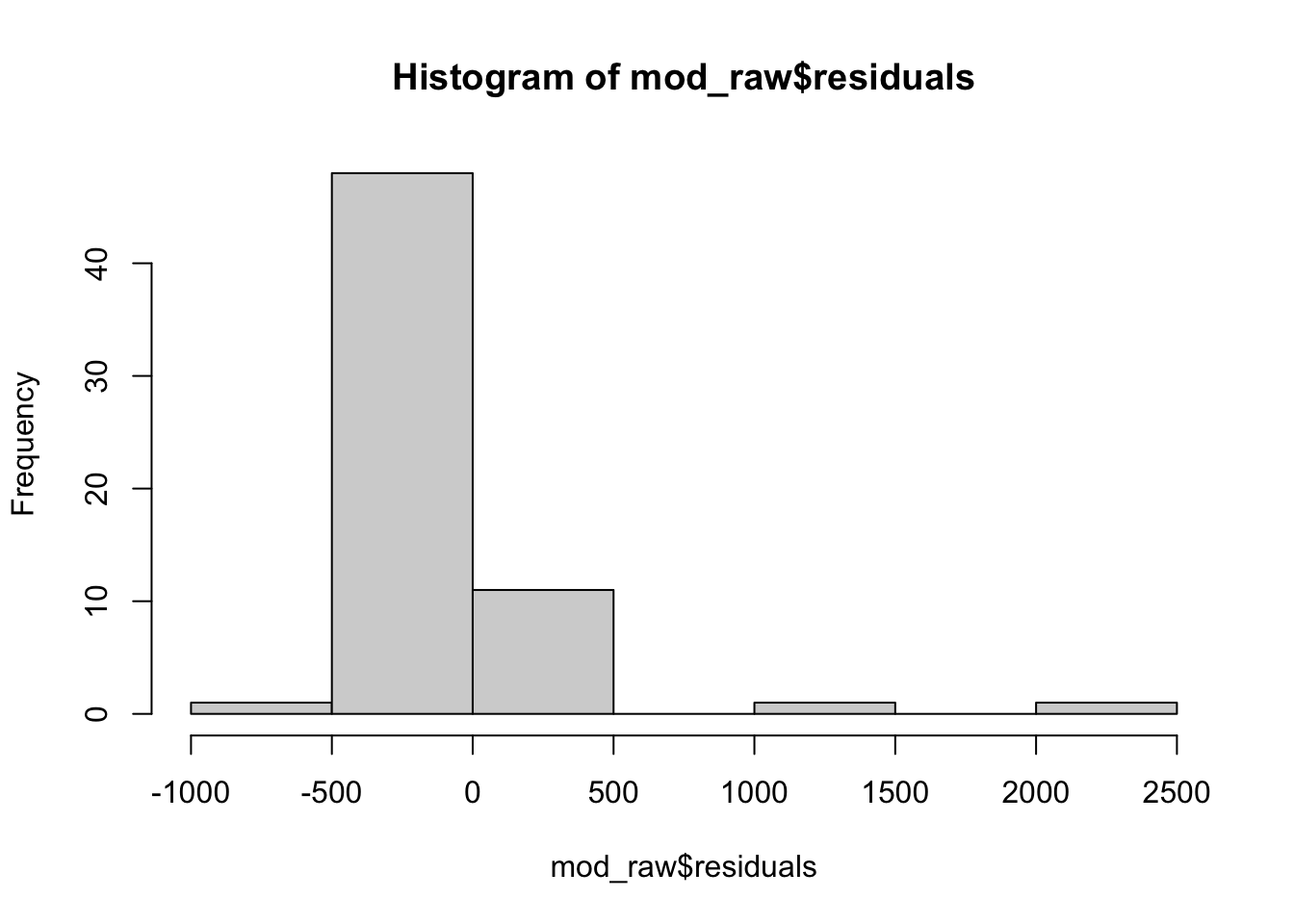

Let’s see what happens when we examine the model output:

summary(mod_raw)


Call:
lm(formula = brain ~ body, data = mammals)

Residuals:
    Min      1Q  Median      3Q     Max 
-810.07  -88.52  -79.64  -13.02 2050.33 

Coefficients:
            Estimate Std. Error t value Pr(>|t|)    
(Intercept) 91.00440   43.55258    2.09   0.0409 *  
body         0.96650    0.04766   20.28   <2e-16 ***
---
Signif. codes:  0 '***' 0.001 '**' 0.01 '*' 0.05 '.' 0.1 ' ' 1

Residual standard error: 334.7 on 60 degrees of freedom
Multiple R-squared:  0.8727,    Adjusted R-squared:  0.8705 
F-statistic: 411.2 on 1 and 60 DF,  p-value: < 2.2e-16

Transform the data + re-fit the model

# Use ggplot to examine the relationship between body weight and brain weight
ggplot(data = mammals, aes(x = log10(body), y = log10(brain))) +
  geom_point() +
  theme_bw()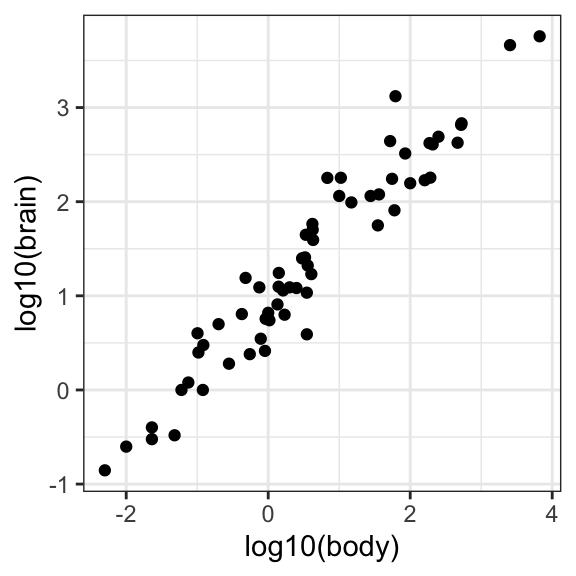

# Use ggplot to examine the histograms for each variable
ggplot(data = mammals, aes(x = log10(body))) +
  geom_density() +
  theme_bw()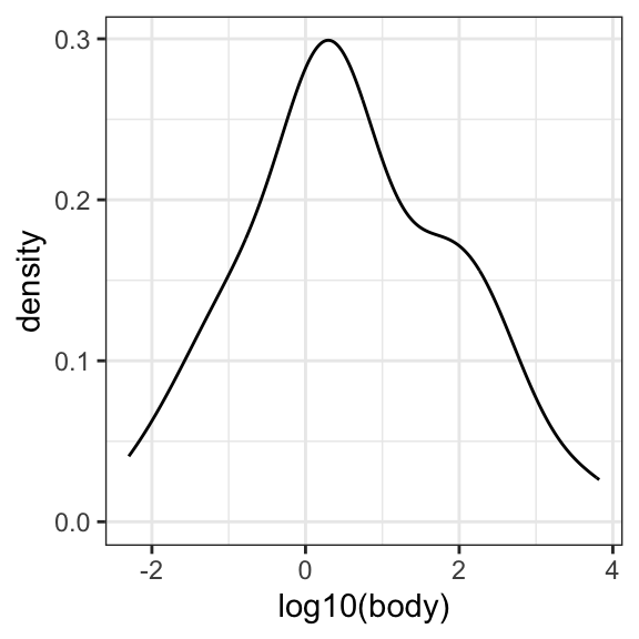

ggplot(data = mammals, aes(x = log10(brain))) +
  geom_density() +
  theme_bw()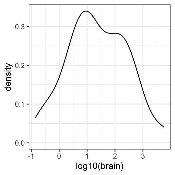

This looks promising, now let’s fit a new model with the transformed variables…

# Fit a new model using log10() to transform both variables
mod_log10 <- lm(log10(brain) ~ log10(body), data = mammals)

par(mfrow=c(2,2))
plot(mod_log10)

hist(mod_log10$residuals)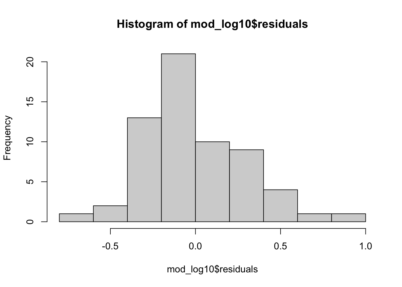

Compare the two models

Let’s compare the model output from the model on the raw data and the model on transformed data:

How would your interpretation of the second model differ from the first? (hint: consider the units of the slope and intercept)

Here is a helpful resource!

# Use `summary` to extract the output from the two models
summary(mod_raw)


Call:
lm(formula = brain ~ body, data = mammals)

Residuals:
    Min      1Q  Median      3Q     Max 
-810.07  -88.52  -79.64  -13.02 2050.33 

Coefficients:
            Estimate Std. Error t value Pr(>|t|)    
(Intercept) 91.00440   43.55258    2.09   0.0409 *  
body         0.96650    0.04766   20.28   <2e-16 ***
---
Signif. codes:  0 '***' 0.001 '**' 0.01 '*' 0.05 '.' 0.1 ' ' 1

Residual standard error: 334.7 on 60 degrees of freedom
Multiple R-squared:  0.8727,    Adjusted R-squared:  0.8705 
F-statistic: 411.2 on 1 and 60 DF,  p-value: < 2.2e-16

summary(mod_log10)


Call:
lm(formula = log10(brain) ~ log10(body), data = mammals)

Residuals:
     Min       1Q   Median       3Q      Max 
-0.74503 -0.21380 -0.02676  0.18934  0.84613 

Coefficients:
            Estimate Std. Error t value Pr(>|t|)    
(Intercept)  0.92713    0.04171   22.23   <2e-16 ***
log10(body)  0.75169    0.02846   26.41   <2e-16 ***
---
Signif. codes:  0 '***' 0.001 '**' 0.01 '*' 0.05 '.' 0.1 ' ' 1

Residual standard error: 0.3015 on 60 degrees of freedom
Multiple R-squared:  0.9208,    Adjusted R-squared:  0.9195 
F-statistic: 697.4 on 1 and 60 DF,  p-value: < 2.2e-16

Graph results

Finally, let’s create a graph to present the results of our final model. This time we will include the error band around the slope.

ggplot(data = mammals, aes(x = log10(body), y = log10(brain))) +
  geom_point() +
  geom_smooth(method = 'lm', se = TRUE) +
  labs(x = "log10 - Body weight (kg)", y = "log10 - Brain weight (g)") +
  theme_bw()

`geom_smooth()` using formula = 'y ~ x'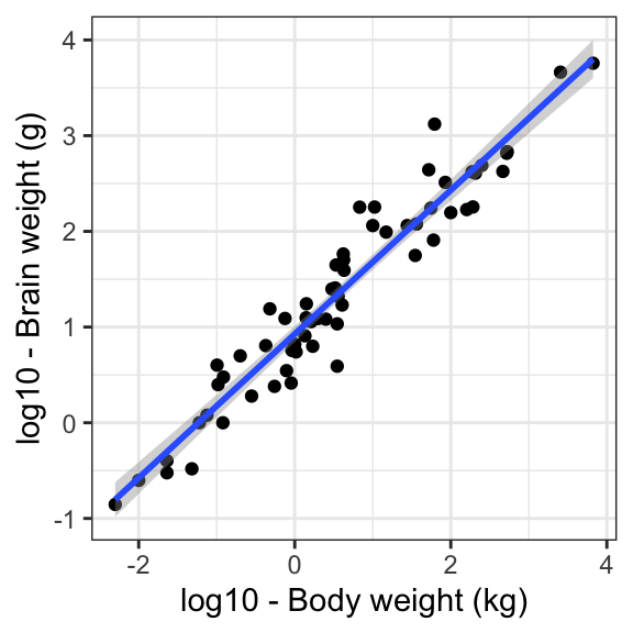

Example 3: Theil-Sen regression

Now let’s look at an example where assumptions are not so clearly met and instead of transformation we take a different approach to the model all together - using a non-parametric alternative called Theil-Sen Regression. We will use the dataset from Tuesday’s lab (Garvin et al. 2006), but look at a slightly different question:

How is does zinc content differ depending on year of variety release?
Predictor (Independent): year
Response (Dependent): seed_Zn_ug_g

garvin <- read.csv("./data/Garvin_2006_data.csv")
str(garvin)

'data.frame':   14 obs. of  3 variables:
 $ year        : int  1919 1942 1944 1964 1967 1970 1978 1982 1984 1992 ...
 $ yield_kg_ha : num  3022 3066 3261 4016 3365 ...
 $ seed_Zn_ug_g: num  26.3 25.5 21.7 22.6 23 ...

Preliminary graphs

# CODE: Use ggplot to examine the relationship between year of release and zinc
 ggplot(data = garvin, aes(x = year, y = seed_Zn_ug_g)) +
  geom_point() +
  geom_smooth(method = 'loess', se = FALSE) +
  theme_bw()

`geom_smooth()` using formula = 'y ~ x'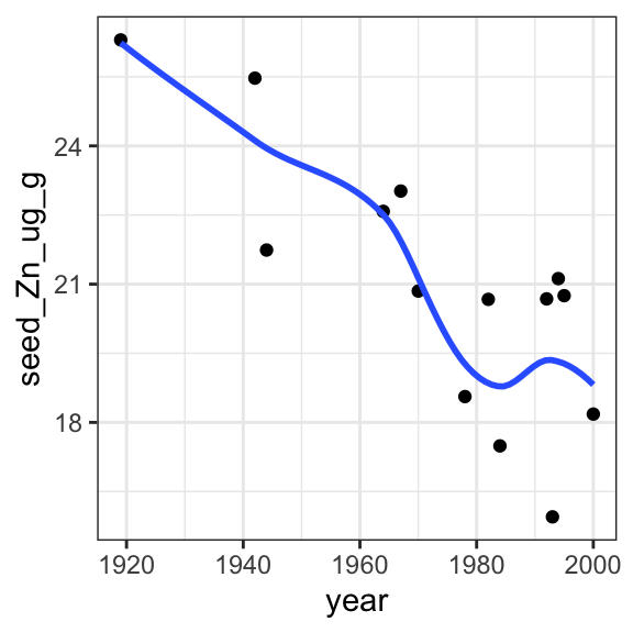

# CODE: Use ggplot to examine the histograms for each variable
 ggplot(data = garvin, aes(x = year)) +
  geom_density() +
   theme_bw()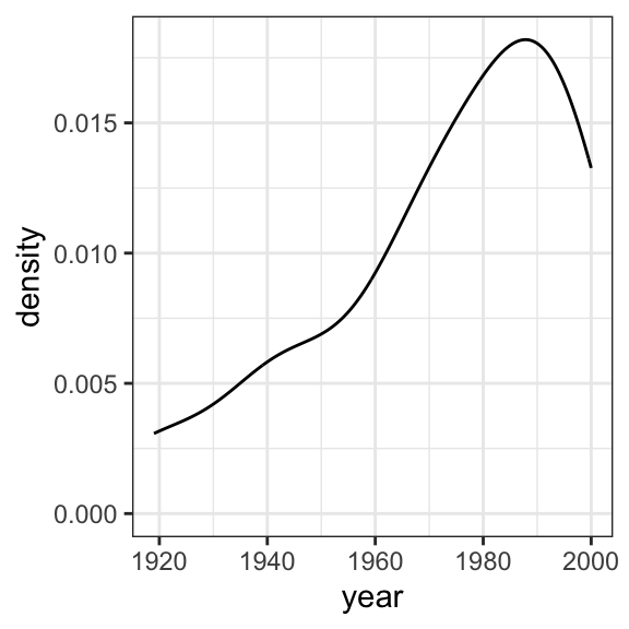

 ggplot(data = garvin, aes(x = seed_Zn_ug_g)) +
  geom_density() +
   theme_bw()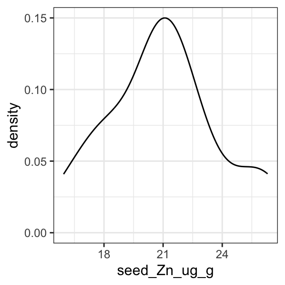

Fit the linear regression model + assess assumptions

Now let’s see what happens when we fit a linear model to these data.

# CODE: Use 'lm' to fit a linear regression model of zinc content as a function of year
mod_raw <- lm(seed_Zn_ug_g ~ year, data = garvin)

# CODE: Use 'plot' and 'hist' to generate diagnostic plots of the residuals from the model
par(mfrow = c(2,2))
plot(mod_raw)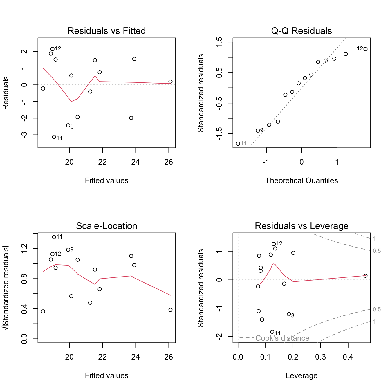

hist(mod_raw$resid)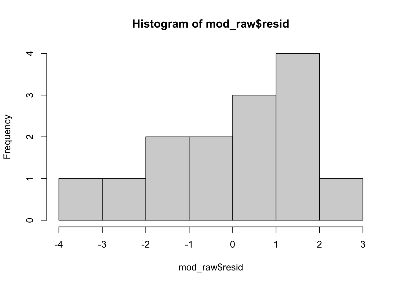

Use Theil-Sen regression to fit an alternative model

# Fit a new model using function `mblm` (median-based linear models)
mod_med <- mblm(seed_Zn_ug_g ~ year, data = garvin)

# We do not look at the distribution of residuals because this method does not make assumptions about the distribution of the residuals

Compare the two models

# Use `summary` to extract the output from the two models
summary(mod_raw)


Call:
lm(formula = seed_Zn_ug_g ~ year, data = garvin)

Residuals:
   Min     1Q Median     3Q    Max 
-3.116 -1.550  0.377  1.510  2.150 

Coefficients:
             Estimate Std. Error t value Pr(>|t|)    
(Intercept) 208.63105   41.36964   5.043 0.000288 ***
year         -0.09512    0.02096  -4.537 0.000682 ***
---
Signif. codes:  0 '***' 0.001 '**' 0.01 '*' 0.05 '.' 0.1 ' ' 1

Residual standard error: 1.814 on 12 degrees of freedom
Multiple R-squared:  0.6317,    Adjusted R-squared:  0.601 
F-statistic: 20.58 on 1 and 12 DF,  p-value: 0.0006815

summary(mod_med)


Call:
mblm(formula = seed_Zn_ug_g ~ year, dataframe = garvin)

Residuals:
    Min      1Q  Median      3Q     Max 
-4.0374 -2.5898 -0.7665  0.3538  1.2347 

Coefficients:
             Estimate       MAD V value Pr(>|V|)   
(Intercept) 223.38411  74.75111     105  0.00109 **
year         -0.10206   0.03911       0  0.00109 **
---
Signif. codes:  0 '***' 0.001 '**' 0.01 '*' 0.05 '.' 0.1 ' ' 1

Residual standard error: 2.152 on 12 degrees of freedom

confint(mod_med, level = 0.95)

                  0.025        0.975
(Intercept) 140.2280043 273.80303768
year         -0.1283798  -0.06004539

Graph results

Theil-Sen regression does not have a built in function in geom_smooth, so we’ll need to take a different approach to fitting our trendline

# To see how the coef() function works, check this out:
coef(mod_med)

(Intercept)        year 
223.3841111  -0.1020556

# Rather than use geom_smooth, we will use geom_abline (use help file to see argument!)
# the function coef() extracts coefficients from the model
ggplot(data = garvin, aes(x = year, y = seed_Zn_ug_g)) +
  geom_point() +
  geom_abline(intercept = coef(mod_med)[1], slope = coef(mod_med)[2], color = "blue") +
  labs(x = "Year of variety introduction", y = "Zinc content (ug/g)") +
  theme_light()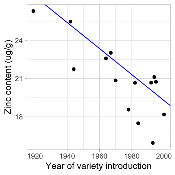

How similar is it to the OLS linear regression line?

# Here is the graph with the standard regression line
ggplot(data = garvin, aes(x = year, y = seed_Zn_ug_g)) +
  geom_point() +
  geom_smooth(method = "lm") +
  labs(x = "Year of variety introduction", y = "Zinc content (ug/g)") +
  theme_light()

`geom_smooth()` using formula = 'y ~ x'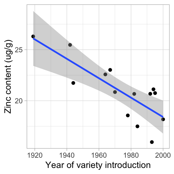

sessionInfo()

R version 4.3.2 (2023-10-31)
Platform: x86_64-apple-darwin20 (64-bit)
Running under: macOS Monterey 12.4

Matrix products: default
BLAS:   /Library/Frameworks/R.framework/Versions/4.3-x86_64/Resources/lib/libRblas.0.dylib 
LAPACK: /Library/Frameworks/R.framework/Versions/4.3-x86_64/Resources/lib/libRlapack.dylib;  LAPACK version 3.11.0

locale:
[1] en_US.UTF-8/en_US.UTF-8/en_US.UTF-8/C/en_US.UTF-8/en_US.UTF-8

time zone: America/New_York
tzcode source: internal

attached base packages:
[1] stats     graphics  grDevices utils     datasets  methods   base     

other attached packages:
 [1] mblm_0.12.1     MASS_7.3-60     lubridate_1.9.3 forcats_1.0.0  
 [5] stringr_1.5.1   dplyr_1.1.4     purrr_1.0.2     readr_2.1.5    
 [9] tidyr_1.3.0     tibble_3.2.1    ggplot2_3.4.4   tidyverse_2.0.0

loaded via a namespace (and not attached):
 [1] sass_0.4.8        utf8_1.2.4        generics_0.1.3    lattice_0.21-9   
 [5] stringi_1.8.3     hms_1.1.3         digest_0.6.34     magrittr_2.0.3   
 [9] timechange_0.3.0  evaluate_0.23     grid_4.3.2        fastmap_1.1.1    
[13] Matrix_1.6-1.1    rprojroot_2.0.4   workflowr_1.7.1   jsonlite_1.8.8   
[17] promises_1.2.1    mgcv_1.9-0        fansi_1.0.6       scales_1.3.0     
[21] jquerylib_0.1.4   cli_3.6.2         rlang_1.1.3       splines_4.3.2    
[25] munsell_0.5.0     withr_3.0.0       cachem_1.0.8      yaml_2.3.8       
[29] tools_4.3.2       tzdb_0.4.0        colorspace_2.1-0  httpuv_1.6.13    
[33] vctrs_0.6.5       R6_2.5.1          lifecycle_1.0.4   git2r_0.33.0     
[37] fs_1.6.3          pkgconfig_2.0.3   pillar_1.9.0      bslib_0.6.1      
[41] later_1.3.2       gtable_0.3.4      glue_1.7.0        Rcpp_1.0.12      
[45] highr_0.10        xfun_0.41         tidyselect_1.2.0  rstudioapi_0.15.0
[49] knitr_1.45        farver_2.1.1      nlme_3.1-163      htmltools_0.5.7  
[53] labeling_0.4.3    rmarkdown_2.25    compiler_4.3.2

Linear regression examples

Environmental Data Analysis, Spring 2024

3/28/24

Goals

Example 1: Removing outliers

Examine scatterplot

Fit a linear regression model + assess assumptions

Exclude outliers + re-fit the model

Compare models

Example 2: Transformation

Preliminary plots

Fit a linear regression model + assess assumptions

Transform the data + re-fit the model

Compare the two models

Graph results

Example 3: Theil-Sen regression

Preliminary graphs

Fit the linear regression model + assess assumptions

Use Theil-Sen regression to fit an alternative model

Compare the two models

Graph results